Qiskit: getting started

Qiskit is an open source software development kit (SDK) for working with quantum computation. There are several excellent tutorials for getting started with qiskit, as well as loads of great documentation you can find at qiskit.org. The following walks through some of the very basics including how to create quantum circuits, simulate measurments, and work with state vectors.

Creating quantum circuits

from qiskit import QuantumCircuit

First, we create a 3-qubit quantum circuit:

qc = QuantumCircuit(3)

Next, we add some gates and draw the resulting circuit:

qc.x(0)
qc.h(2)
qc.cx(0,2)
qc.cx(1,2)
qc.draw(output='mpl')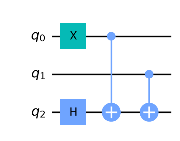

Measurements

We can simulate a measurement, but first we need to import a simulator:

from qiskit.providers.aer import QasmSimulator

simulator = QasmSimulator()

Measure using a classical register explicitly

One way to measure is to use a circuit having both a quantum and classical register:

circuit = QuantumCircuit(3, 3)

Now, let’s add some gates including some measuments:

circuit.h(0)
circuit.cx(0, 1)
circuit.cx(0, 2)
circuit.measure([0,1,2], [0,1,2])
circuit.draw(output='mpl')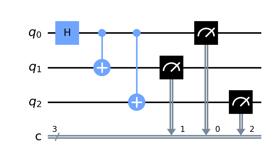

Next, we simulate and count the results:

job = simulator.run(circuit, shots=1000)
result = job.result()
counts = result.get_counts(circuit)
print(counts)

{'000': 469, '111': 531}

We can plot the results using qiskits built in visualization:

from qiskit.visualization import plot_histogram

plot_histogram(counts)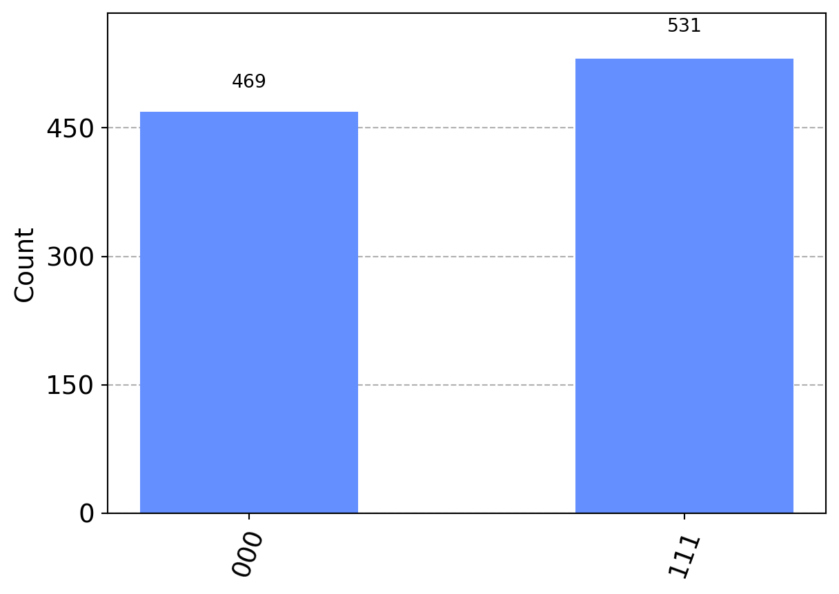

Using the measure_all() method

Alternatively, if we want to measure all the qubits we can use the measure_all() method:

circuit = QuantumCircuit(3)

Now, let’s add some gates including some measuments:

circuit.h(0)
circuit.cx(0, 1)
circuit.cx(0, 2)
circuit.measure_all()
circuit.draw(output='mpl')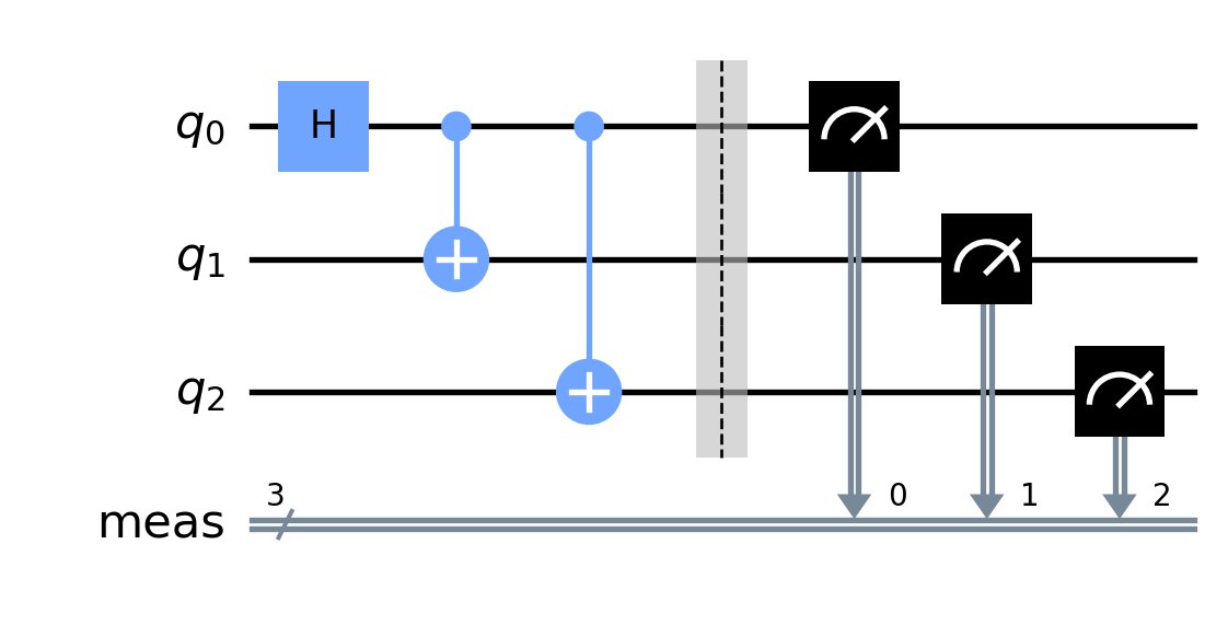

We should see similar results:

job = simulator.run(circuit, shots=1000)
result = job.result()
counts = result.get_counts(circuit)
print(counts)

{'000': 490, '111': 510}

Of course, this will only work if we want to measure all the qubits in the output state of the circuit.

Circuit orientation

Qiskit orients circuits so that the qubits \(q_0, q_1,\ldots, q_{n-1}\) labelling the circut from top to bottom correspond to the input state \(|q_{n-1}\cdots q_1q_0\rangle\). To see this, let’s create a simple gate that maps \(|000\rangle\mapsto|100\rangle\).

circ = QuantumCircuit(3)
circ.x(2)
circ.measure_all()
circ.draw(output='mpl')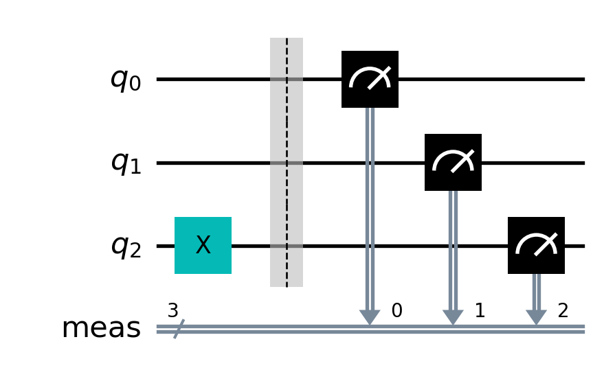

To see that the circuit above does the trick, let’s measure:

job = simulator.run(circ, shots=1000)
result = job.result()
counts = result.get_counts(circ)
print(counts)

{'100': 1000}

I prefer the flipped orientation where the top qubit in the circuit corresponds to the left qubit in the tensor product. To have qiskit draw circuits with my prefered orientation, we simply pass reverse_bits=True to the draw() method:

circ.draw(output='mpl', reverse_bits=True)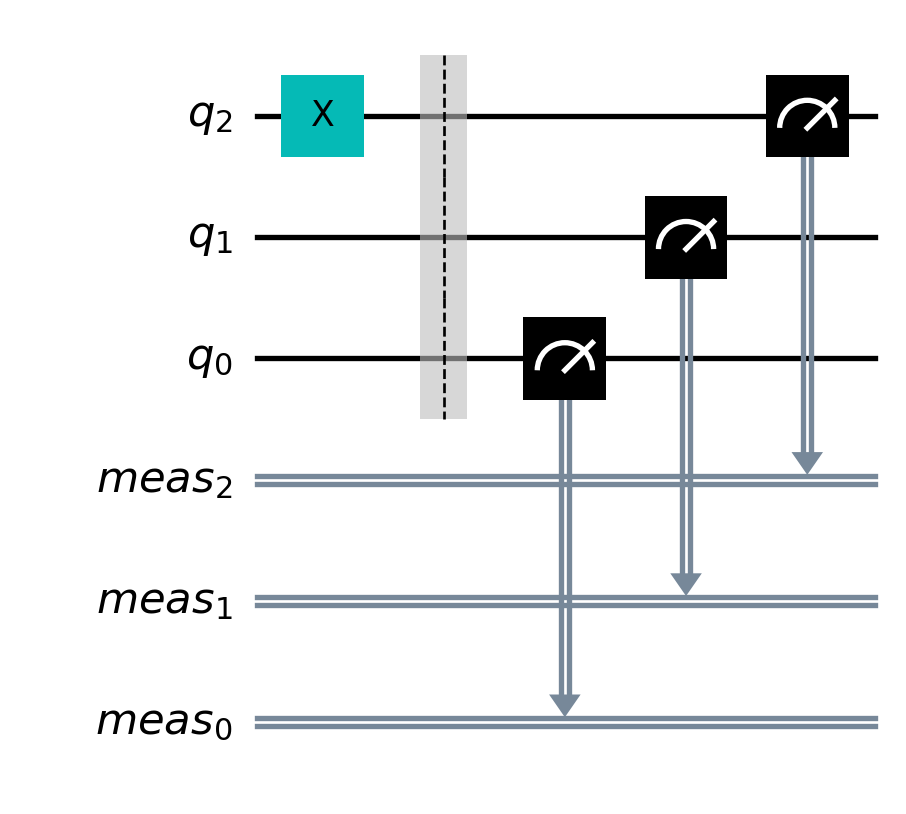

job = simulator.run(circ, shots=1000)
result = job.result()
counts = result.get_counts(circ)
print(counts)

{'100': 1000}

State vectors and Bloch spheres

We can use qiskits Statevector object work with \(n\)-qubit states.

from qiskit.quantum_info import Statevector

For example, the following creates the state \(|7\rangle\) for a 4-qubit register:

state = Statevector.from_int(7, 2**4)
state.draw('latex')

\[ |0111\rangle\]

We can visualize the state \(|7\rangle\) on a register of Bloch spheres as follows:

from qiskit.visualization import plot_bloch_multivector

plot_bloch_multivector(state, reverse_bits=True)

We can run this state through a quantum circuit as in the following example:

qc = QuantumCircuit(4)
qc.h(1)
qc.h(2)
qc.cx(0, 2)
qc.swap(1,3)
qc.draw(output='mpl', reverse_bits=True)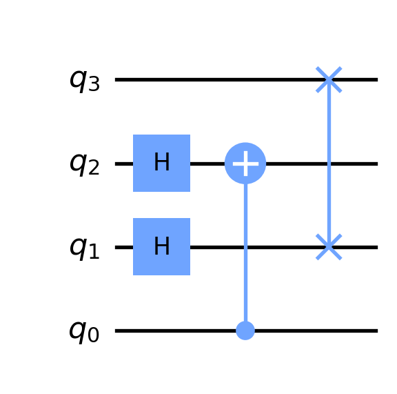

state = state.evolve(qc)
state.draw('latex')

\[- \frac{1}{2} |0001\rangle+\frac{1}{2} |0101\rangle+\frac{1}{2} |1001\rangle- \frac{1}{2} |1101\rangle\]

Finally, let’s look at this state using Bloch spheres:

plot_bloch_multivector(state, reverse_bits=True)